
What does the cost of debt tell us about the cost of equity—part two
How can data on the cost of debt be used to improve estimates of the cost of equity? A previous article on this topic, published in May 2023, explained that as a senior claim on the assets, the debt risk premium should be lower than the risk premium on unlevered equity at any level of gearing. But can a tighter (i.e. higher) lower bound on the unlevered equity risk premium be derived?
The return that investors expect when they commit equity capital to a company cannot be directly observed. In contrast, the return required by providers of debt finance is contractually agreed. When estimating the cost of equity for a company, it is therefore natural to consider what information can be gleaned from the cost of debt of that company.
The previous Oxera article introduced the concept of comparing the risk premium on unlevered equity, i.e. the asset risk premium (ARP), with the risk premium on debt, i.e. the debt risk premium (DRP).1 As a senior claim on the assets, the DRP should be lower than the ARP at any level of gearing. This provides an initial lower bound on estimates of the ARP, and thereby bounds the cost of equity.
Further insight can be obtained from the comparison of the ARP to the DRP by considering the relationship between risk premia and gearing. This enables the derivation of a tighter (i.e. higher) lower bound to the ARP that is valid for most practical purposes, and relies on no more information than the company’s cost of debt and its level of gearing. How is this lower bound derived? To explain, we look at a practical application below.
What is the lower bound on the asset risk premium?
The DRP is defined as the expected return on debt in excess of the risk-free rate, where the expected return on debt is lower than the promised return on debt by an amount equal to the ‘expected loss’ (probability of default multiplied by the loss given default). The DRP should be close to zero when gearing is close to zero because the risk to lenders will be minimal. The DRP increases with gearing, as lenders expect a higher return in compensation for bearing the higher risk of financial distress. As gearing approaches 100%, the DRP will approach the ARP (i.e. the unlevered cost of equity minus the risk-free rate), as the company would now be financed almost entirely by debt. At no point in this relationship would the DRP ever exceed the ARP.
By the same logic, the minimum level of the ARP–DRP differential can be deduced by using the relationship between the risk premia and gearing for a specific company. This relationship is illustrated in Figure 1.
Figure 1 The relationship between risk premia and gearing
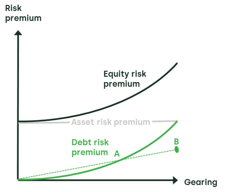
The DRP is associated with the company’s level of gearing, and is depicted by point A in the figure. The relationship between the DRP and gearing is also shown.
The DRP is usually assumed to be a convex function of gearing, and estimating this function is not straightforward. However, if analysis is undertaken assuming a linear relationship between DRP and gearing, the figure shows that extrapolating the line connecting the origin and point A provides a prediction of the debt risk premium at 100% gearing (point B) that will be lower than the ARP.
The slope of the linear relationship is given by dividing the observed DRP by the observed gearing (point A). Multiplying the slope by hypothetical gearing of 100% provides the extrapolation of the DRP to point B. For example, if a DRP of 100bp is observed at 50% gearing (point A), then a DRP of 200bp is predicted at point B.
A linear extrapolation to 100% gearing will underestimate the DRP, and hence the lower bound on the asset risk premium if debt risk is a convex function of gearing. Therefore, the risk premium on unlevered equity should be strictly greater than the risk premium on debt divided by gearing. This provides a tighter (i.e. higher) lower bound on estimates of the cost of equity compared with using the directly observed DRP as the benchmark.
Practical considerations
Applying the framework requires two variables to be measured: gearing and the debt risk premium.
Figure 1 suggests that the framework will be most accurate when producing estimates of the ARP for companies that are highly geared—as this is where the gap between the DRP and the ARP is smallest. However, where the high gearing is also associated with a low credit rating, compensation for the expected loss on such debt will be a relatively large component of the promised return on debt. Indeed, the promised return on debt will exceed the expected return on assets as gearing approaches 100%. In such cases, extra attention should be paid to the assumption for expected loss, which can be estimated based on historical rates of default and loss given default.
The reliance on accurate estimates of expected loss is reduced when considering companies with low levels of gearing and high credit ratings, where the probability of default is low. However, this creates a different problem. Figure 1 shows that the curvature of the DRP function is low when gearing is low—therefore extrapolation of the DRP from such points will project a line that is close to horizontal. At a gearing level approaching 100%, there will be a large gap between the ARP and the linearly extrapolated DRP. Although this provides a tighter lower bound on ARP than using DRP alone (the latter being suggested by DRP having to always be below ARP), the true ARP could be significantly higher than this bound.
The preceding discussion implies that estimates of the ARP will be better when they are based on companies with a relatively high level of gearing and a relatively low probability of default—for example, companies with investment-grade credit ratings.
How has the lower bound for the cost of equity varied over time?
Figure 2 shows yield spreads over the last five years on indices of BBB-rated corporate bonds denominated in EUR and GBP. Spreads are calculated relative to German bunds and UK gilts respectively.2 The averages over the last five years are 161bp and 173bp.3 Assuming expected loss of 30bp,4 the average DRP was 131bp and 143bp.
Figure 2 Corporate bond spreads (%)
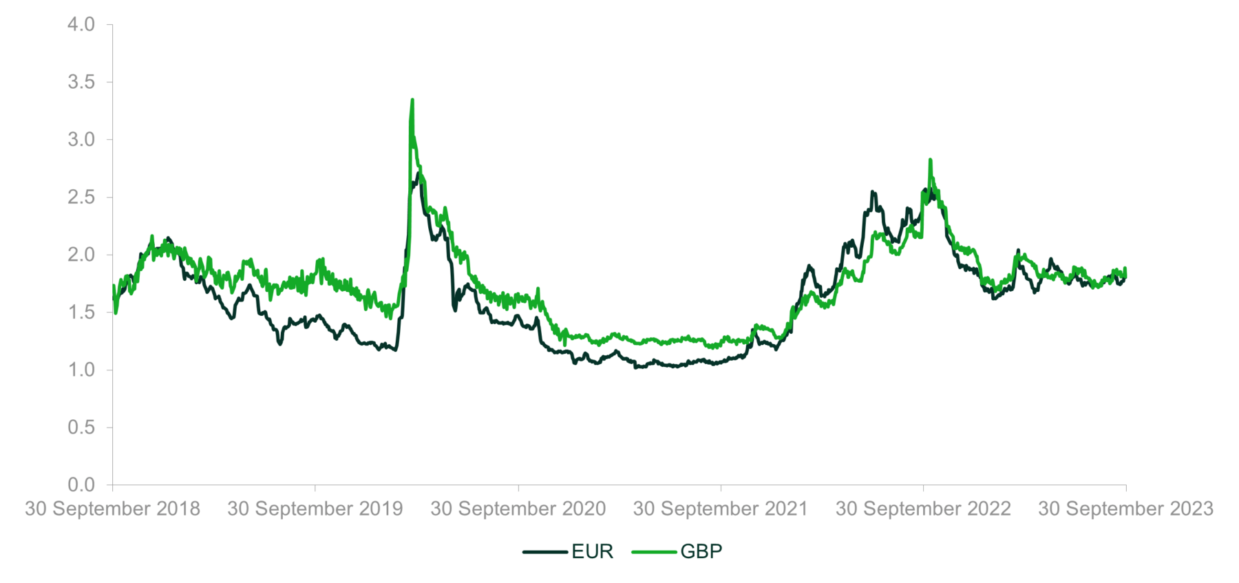
Source: Oxera analysis of data from IHS Markit and Eikon.
Assuming gearing of 60% net debt to enterprise value would provide lower bounds of 218bp and 238bp on the ARP.
The lower bounds on the ARP can be relevered and added to the government bond yield to give lower bounds of 3.83% (EUR) and 5.27% (GBP) on the nominal cost of equity for BBB-rated companies. These estimates are averages over the past five years.
Using yields and spreads as at 30 September 2023 instead of the five-year averages provides lower bounds on the nominal cost of equity of 6.79% (EUR) and 8.41% (GBP).
These calculations are presented in Table 1.
Table 1 Calculation of the lower bound on the nominal cost of equity
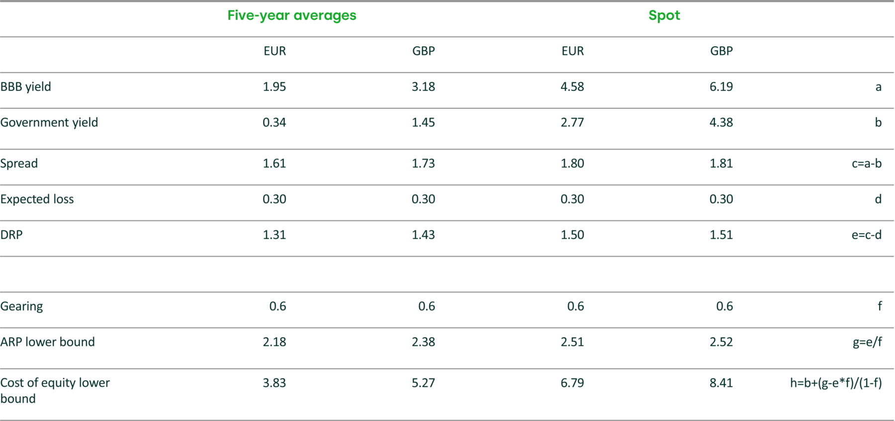
Source: Oxera analysis of data from IHS Markit and Eikon.
Analysis has been presented at a high level of aggregration based on average BBB-rated corporate bond yields and an assumed gearing level of 60%, and should be adapted to the circumstances of the specific case. The analysis has also been simplified, for example by assuming that government bond yields are an unbiased estimate of the risk-free rate, and factors such as the convenience yield are not accounted for.
Can estimates of the cost of equity be improved?
Applying the CAPM to calculate the cost of equity requires estimates of the equity beta, the market equity risk premium and the risk-free rate. A complementary approach to estimating the cost of equity is to draw on additional evidence from the debt markets. The conceptual relationship between the pricing of a debt claim and the risk of the underlying asset can be used to infer a lower bound for the cost of equity, and therefore improve the precision of estimates derived from other methods.
1 Oxera (2023), ‘What does the cost of debt tell us about the cost of equity?’, Agenda, 31 May. Oxera (2019), ‘Risk premium on assets relative to debt’, 25 March, and Oxera (2020), ‘Asset risk premium relative to debt risk premium’, 4 September.
2 Strictly speaking, the calculation should also account for an estimate of the convenience yield embedded in government bond yields. This step is omitted here for ease of exposition.
3 The cut-off date is 30 September 2023.
4 Expected loss is calculated using annualised default rate and loss given default. The annualised default rate is derived from the cumulative default rates (CDR) from Table 8 of Feldhütter, P. and Schaefer, S. M. (2018), ‘The Myth of the Credit Spread Puzzle’, Review of Financial Studies, 31:8, pp. 2897–942. Loss given default is assumed to be 40%, based on Moody’s (2019), ‘Annual default study: Defaults will rise modestly in 2019 amid higher volatility’.
Contact

Peter Hope, CFA
PartnerGuest author
Professor Julian Franks
Contributors
Related
Related

No water, no growth: tackling inefficient business water demand
Water is not typically thought of as a constraint on economic growth in England. Yet that is precisely what it is becoming. Commercial growth and new developments are being turned away because there is insufficient water to serve them. Some water companies are already exercising their powers to refuse… Read More

The energy trilemma in focus: the price of dependence
Europe’s approach to energy policy has been in transition since the 2022 energy crisis laid bare the continent’s dependence on imported fossil fuels. More recently, the outbreak of war in the Middle East and the subsequent disruption to global oil and gas markets have caused further challenges. This article… Read More