Turning down the volume: estimating cost of capital in the presence of noise

For the last 30 years, the cost of capital has been a central element of the price-control frameworks applied across regulated industries. It typically comprises 30% to 40% of the amount that regulated infrastructure companies are allowed to charge their customers.[1]

Beta is one element involved in estimating the cost of capital. Despite it being a low number in absolute terms, varying the beta can have a significant impact on the implied value of an asset. For example, in a recent court case involving the valuation of Rural/Metro, a publicly traded US ambulance provider, using two different acceptable methods to estimate the beta resulted in a value difference of over $100m.[2]

Some background

Estimating the cost of capital overall is not straightforward. It has been subject to extensive debate, in part because it requires the determination of the unobservable fair remuneration for equity investors. Nevertheless, regulators around the world mostly agree about using the capital asset pricing model (CAPM) to estimate the required returns on equity.

The CAPM states that the equilibrium required rate of return on equity equals the ‘risk-free’ rate of return,[3] plus a premium to reflect the relevant risk. This risk premium is a product of the equity risk premium[4] for holding a diversified portfolio of shares, plus a measure of the sensitivity of the particular equity to overall market movements (this latter measure is the beta). The box below provides a summary of the CAPM. This article assumes that the CAPM is the true representation of required return on equity.

There are estimation difficulties with all the parameters in the CAPM, not least because a regulator needs to take a forward-looking view while using largely historical information.

First, determining the risk-free rate is challenging due to deterioration of yields on safe sovereign bonds, coupled with spikes in yields for a number of European governments and the future uncertainty around these yields. UK regulators have therefore tended to err on the side of caution, perhaps to ensure that the regulated entities have sufficient allowance to cover their financing costs. This is shown in Figure 1.

Figure 1   Regulatory determinations on the risk-free rate vs UK gilt yields

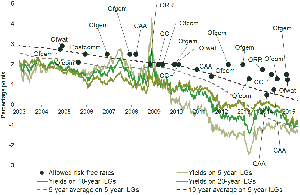
Note: ILG, index-linked gilt. CAA, Civil Aviation Authority. ORR, Office of Rail and Road (formerly the Office of Rail Regulation). CC, Competition Commission.

Source: Oxera.

Second, estimating the equity risk premium involves quantifying the extra returns required by investors for taking on the general risks associated with investing in the equity market. Typically, such estimates are made by reference to historical data on market performance, although this evidence can be of limited statistical validity in certain markets, both because it is backward-looking and because the observed performance may not always reflect the direction of the level of risk. Alternative methods are therefore also used, such as surveys in which market practitioners are asked to give their view on the equity risk premium.

Beta reflects the sensitivity of a given equity to market movements.[5] In short, it captures what economists call ‘systematic risk’—risk that cannot be diversified. For example, an ice-cream stall typically performs well on sunny days, and less well on rainy days. An umbrella stall does well on rainy days, but not on sunny days. By investing in both, an investor can diversify some of their total risk—but not all of it, because if there is a massive economic downturn people will buy both less ice cream and fewer umbrellas, regardless of the weather. Because this systematic risk cannot be eliminated, investors need to be compensated for it—with the scale of the required compensation being proportionate to the beta.

There are a number of reasons why estimating this parameter is particularly challenging for regulators. First, if a company is not public (i.e. traded on a stock exchange), it is not possible to track its sensitivity to market movements. In such cases, a set of comparable public companies is analysed instead. But even if a company is public, there are further challenges.

In most cases the equity price observed on the market refers to a company as a whole, and may not closely reflect its regulated activities. Beta estimates are also typically derived by reference to historically observed movements in equity prices relative to the stock market as a whole. In any statistical analysis of this type, it is preferable for the sample to contain a large number of observations. However, historical information from the distant past may be of limited relevance, as a company may have gone through significant changes since that time, such as disposing of certain activities or exiting markets.

There is therefore often a trade-off between including as many observations as possible and ensuring that these are fully relevant. Regulators typically look at one-year, two-year and five-year betas—that is, information from one to five years in the past.

Equity prices can also be measured at different frequencies—for example, at the end of each month, week, day or even minute. While using a higher frequency increases the number of observations, it is unclear how far intra-day price oscillations reflect the fundamental risk characteristics of a company. In particular, using higher frequencies can introduce market microstructure noise into the estimation.[6] Regulators therefore often use daily, weekly and monthly frequencies.

In an ideal world, all of these different approaches would give similar results. In fact, significant differences are found depending on the basis of the calculation.

The example below considers an objective mathematical method for ‘cleansing’, or adapting, the underlying data used to estimate betas. This can help to make sense of the sometimes conflicting empirical evidence stemming from what initially appear to be equally valid approaches.

One of the major difficulties with estimating beta is that equity price data is subject to noise—that is, equity prices may deviate from their equilibrium values (in this case, CAPM-implied prices). This can happen in response to news announcements or one-off, company-specific events.[7] By definition, noise does not represent systematic risk, and should not influence the beta estimation result.

The problem with noisy events is that they can sometimes skew the beta estimate. One way to mitigate this is by manually identifying unusual events by monitoring news coverage, and either adjusting or excluding the corresponding price movements altogether. This would exclude market overreactions that do not reflect the fundamental value of the asset. The drawback of this approach is that it is time-consuming, statistically unreliable, and potentially open to manipulation.

There is, however, a more structured way. This involves dividing the dataset into groups and assigning less weight to (apparently) more noisy groups and more weight to less noisy groups, rather than treating all observations equally. This is illustrated in the following example.

Beta puzzle

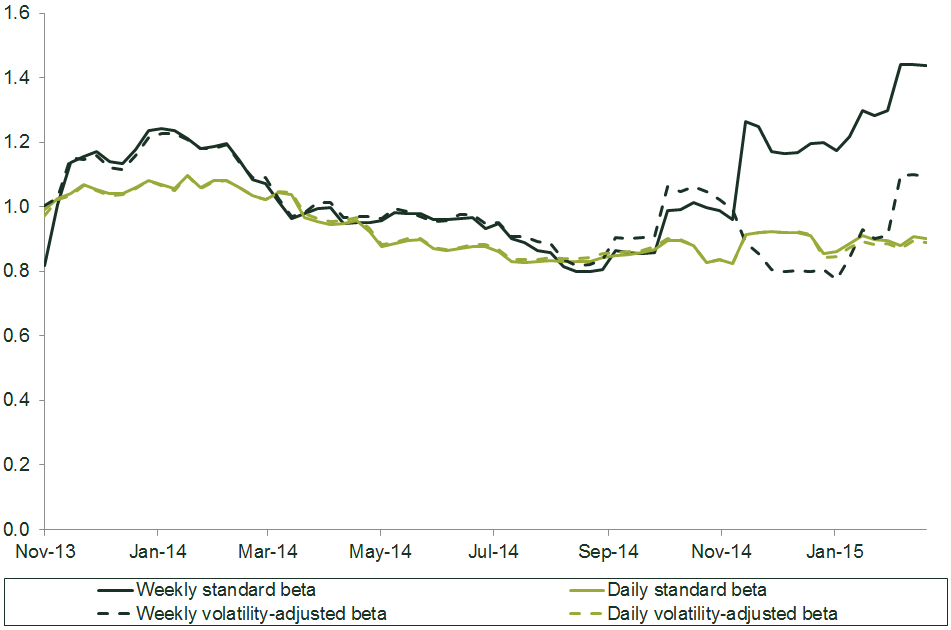
Figure 2 shows two-year weekly and daily equity betas for a regulated infrastructure provider.

The data prior to November 2014 produced similar estimates from daily and weekly data. However, since November 2014, the weekly and daily beta estimates have diverged significantly.

Figure 2   Two-year daily and weekly equity betas

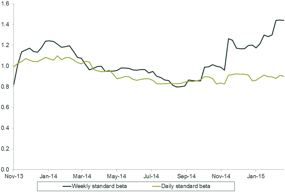
Source: Oxera analysis based on Datastream.

The regulator needs to decide how to tell which beta estimate—daily or weekly—should be attributed more weight. One potential solution involves using techniques from quantitative finance, in which the behaviour of asset price movements is explained in a systematic way.

A bit of quantitative finance

It has long been recognised that the volatility of price oscillations changes from period to period—i.e. from day to day or from week to week. Empirical evidence suggests that, up to a point, these changes can be explained by market behaviour in the recent past.[8] In particular, it has been established that periods following stock price declines are associated with disproportionately high volatility. That is, all else being equal, a price change of -5% is expected to be followed by larger volatility than a price change of +5%. This is sometimes referred to as the leverage effect.[9]

The leverage effect can be incorporated into beta estimation in order to make the beta estimate more robust. (This is just one way to address the problem—other approaches are mentioned at the end of this article.)

Because the CAPM states that the required return on equity reacts symmetrically to a market movement, the leverage effect is attributed to idiosyncratic return—i.e. to noise. The aim of beta estimation is to strip out the noise from the observed equity movements.[10] Thus, if we know that a given day or week was particularly noisy, we should attribute less weight to this observation when determining the beta. To demonstrate how such an approach can work in practice, the following steps were used to estimate the hypothetical volatility-adjusted beta for the firm in Figure 2.

First, the two-year sample of weekly price movements was broken down into the weeks following a week in which the market declined, and those following a week of market growth. Figure 3 illustrates the weekly data sample and how the dataset might be divided in this way.

The bright-green dot in the top-right quadrant shows that, during that week, the market grew by c. 1%, while the equity in question grew by around 10%. The large size of the dot means that the market also grew in the previous week.

The red dot in the bottom-left quadrant shows that, during that week, the market declined by almost 2%, while the equity in question dropped by over 10%. The small size of the dot means that the market also declined in the previous week.

Figure 3   Equity weekly returns against market weekly returns

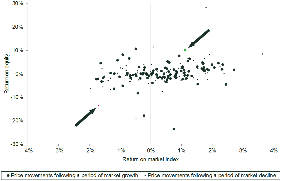
Source: Oxera analysis based on Datastream.

Next, a simple model is estimated that assumes that the volatility[11] of noise is different for the two datasets defined above. The estimation attributes weights to the two datasets inversely to their relative noisiness.[12] This is shown in Figure 4.

Figure 4   Volatility adjustment

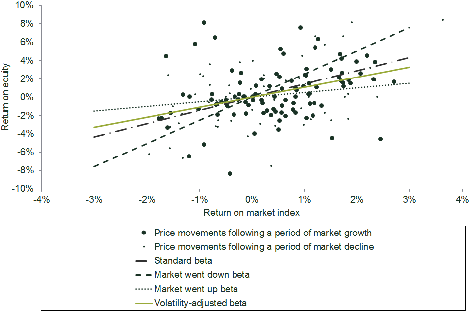
Source: Oxera analysis based on Datastream.

The ‘market went down beta’ is a standard beta estimated using only those weeks that followed a market decline. This beta estimate equals 2.5. The ‘market went up beta’ is a standard beta estimated using only those weeks that followed a market growth, and amounts to 0.5. The striking difference between the two estimates illustrates the significance of the leverage effect.[13] The standard beta derived from the whole sample is 1.4, which falls roughly between the ‘market went down beta’ and the ‘market went up beta’, since it attributes equal weight to all observations.[14]

In contrast, the ‘volatility-adjusted beta’ lies close to 1.1, which is much closer to the ‘market went up beta’. This is because the volatility adjustment method recognises that this subset of data is less noisy—i.e. more informative—and gives it greater weight as a result. (In reality, no ‘weighting’ as such occurs—rather, the volatility-adjusted beta estimate is a result of an objective mathematical process.)

Figure 5 compares the standard and volatility-adjusted betas over time. It shows that the observed increase in the standard weekly beta is likely to have been significantly driven by noise at certain data points.

Figure 5   Comparison of volatility-adjusted and standard betas

Source: Oxera analysis based on Datastream.

Given this result, the next step might be to consider why specific data points have been identified as noisy, and assess whether it is right that these data points should be given little weight. This will always require a degree of judgement—but in the context of objective mathematical analysis.

Other methods

The example above is just one way of separating data from noise, and there are other hypotheses about the interaction between market and equity prices and their volatility that can be applied.

An alternative is to use Bayesian-based methods, such as the Kalman filter, which enables the estimation of unobservable variables that also change over time. This procedure assumes a prior view of the world[15] as an input (for example, beta being equal to 1). Each time new information ‘comes in’ (for example, each time new stock and index prices are observed), the prior belief is updated. The degree to which the prior belief changes as a result of new information is determined by how different the prior belief was from the observed data. The advantage of this technique is that it enables changes in beta over time to be observed. It has also been used in many fields outside of economics, such as in navigation control. In contrast to the volatility model, a simple Kalman filter model assumes that beta itself is always changing, but that volatility remains constant. To be precise, the Kalman filter assumes that beta follows an AR(1) process, in that beta tomorrow equals beta today plus a random shock, with a constant variance.

Both techniques can add value and need to be considered in the context of the problem at hand. Moreover, both approaches can be generalised to include more sophisticated forms of dependence between equity prices, their volatilities and beta.

Conclusion

Cost of capital estimation is a central part of both the regulatory process and commercial project evaluation, but it is also subject to significant uncertainty affecting all parameters of the CAPM. One of the difficulties in estimating the beta is the often materially divergent values that result from datasets of different duration and estimation frequency. While there may be underlying reasons for such divergence, there are also opportunities to remove uncertainty through established mathematical techniques.

The outcome of such techniques is often to identify and de-emphasise noisy data. Alongside this, the dataset itself should be examined to ensure that this de-emphasis can be justified and explained by reference to the root causes of unusual (noisy) share price movements.

[1] See, for example, Commission for Energy Regulation (2010), ‘Decision on 2011 to 2015 distribution revenue for ESB Networks Ltd’. Return on capital and incentives comprise over 40% of total revenue.

[2] Supreme Court of the state of Delaware (2015), ‘Appellant RBC capital markets, LLC’s opening brief’, 19 May, p. 59. Indap, S. (2015), ‘Beta max’, Financial Times, 19 June.

[3] The return paid by a risk-free asset, such as a reliable government bond.

[4] That is, return over and above a risk-free rate demanded by investors for holding a basket of equities.

[5] Brealey, R.A., Myers, S.C. and Allen, F. (2008), Principles of Corporate Finance, p. 193.

[6] See, for example, Cartea, Á. and Karyampas, D. (2011), ‘Volatility and Covariation of Financial Assets: A High-Frequency Analysis’, Journal of Banking and Finance, 35:12, December, pp. 3319–34.

[7] Also known as idiosyncratic events.

[8] This does not contradict the efficient market hypothesis, which states that the level of returns is unpredictable.

[9] Also referred to as the news impact effect. For example, see IMF (2014), ‘Global Financial Stability Report. Risk taking, liquidity, and shadow banking: Curbing excess while promoting growth’, October, p. 61; Glosten, L.R., Jagannathan, R. and Runkle, D.E. (1993), ‘On the relation between the expected value and the volatility of the nominal excess return on stocks’, Journal of Finance, 48, pp. 1779–801; Nelson, D.B. (1991), ‘Conditional heteroskedasticity in asset returns: A new approach’, Econometrica, 59, pp. 347–70; and Engle, R.F. and Ng, V.K. (1993), ‘Measuring and testing the impact of news on volatility’, Journal of Finance, 48:5, pp. 1749–78.

[10] Technically, the aim is to separate the systematic return from the excess (or idiosyncratic) return. The former is the ‘fair’ level of return that a company with a given risk profile would be expected to earn, while the latter is a firm-specific deviation, which averages to zero over time.

[11] That is, standard deviation.

[12] It is assumed that excess return is normally distributed. The technique can be generalised to consider other distributions as well.

[13] Statistical tests also confirm that the effect is significant.

[14] That is, to the periods that followed market decline and those that followed market growth. The ultimate impact of an observation on the beta estimate also depends on its value.

[15] That is, a belief about the world before any data is observed.