Finding the right formula: de-levering and re-levering the beta in the CAPM

Should the tax shields of a firm be discounted with the risk-free rate or the cost of debt? Or perhaps the weighted average cost of capital? The answer will affect how the beta parameter in the Capital Asset Pricing Model (CAPM) is adjusted to account for leverage and the resulting estimate of the cost of capital. We look at the models available to de-lever the beta, and highlight the importance of carefully considering their underlying assumptions.

Discount rates are a key input to investment appraisals, asset valuations, profitability assessments and the setting of regulated revenue allowances. The estimation methodology for discount rates incorporates important assumptions about the treatment of leverage and the risks of a firm’s cash flows, which can lead to significantly different results and materially affect the valuation of an asset or the revenue allowance of a regulated firm.

A considerable body of academic literature discusses this topic and proposes a range of solutions to the treatment of leverage and cash flow risk. In this article, we focus on the cost of equity, which captures both asset risk and leverage risk.

The cost of equity is typically estimated using the CAPM, described in the box below.

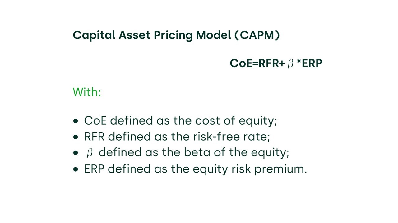
According to the CAPM, the equilibrium required rate of return on equity equals the ‘risk-free’ rate of return, plus a premium to reflect the relevant risk. This risk premium is a product of the equity risk premium—i.e. the premium for holding a diversified portfolio of shares—and the beta parameter, which measures the sensitivity of the particular equity to overall market movements.

For a firm with debt, the equity beta captures both business (or ‘asset’) risk and financial risk, where the latter depends on the company’s capital structure. In order to compare business risk across companies and industries, it is necessary to adjust for financial risk. This process is defined as beta de-levering.

An additional step is necessary to adjust the de-levered beta to the level of leverage of the firm of interest. This secondary step is defined as beta re-levering.

In this article, we explain the underlying assumptions of different beta de-/re-levering formulas and the economic principles behind each specification.

De-levering and re-levering the beta

The different approaches that can be used to de-lever and re-lever betas start from the same principle—that a firm’s value is equal to the present value of its cash flows. However, there are divergences in terms of how tax shields should be discounted depending on the financing strategy of a firm.

Below, we present a summary of the common assumptions that are made in the de-levering and re-levering procedure.

General considerations

In general, the value of a firm can be written as:

Where E is the value of equity, D is the value of debt, A is the present value of the unlevered free cash flows, and TS is the present value of the tax shield, generated by the interest expenses paid on the outstanding debt.

In the context of the CAPM, the following expression can be derived, in which the weighted average of the betas of levered equity and debt is set equal to the weighted average of the betas of the unlevered assets and of the tax shield:

With:

• β_L defined as the levered beta of the company;
•  β_U defined as the unlevered beta or asset beta—i.e. a measure of the equity risk without leverage;
•  β_D defined as the debt beta;
•  β_TS defined as the tax shields beta.

From the equation above we can obtain:

At this point, different assumptions about the long-term financing strategy of a firm and the riskiness of tax shield cash flows lead to different formula specifications.¹ We examine the two special cases in which debt and leverage respectively are assumed to be constant over time.

Constant debt assumption: the Hamada equation

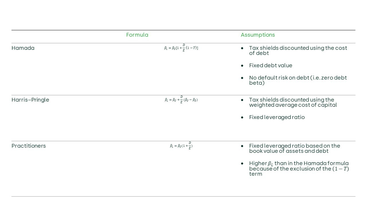
The Hamada formula² assumes that firms follow a constant debt policy in monetary terms—i.e. fixed D. Further, it assumes that the risk associated with the tax shield is equivalent to the risk associated with interest payments (i.e. β_TS = β_D), and therefore that the cost of debt is used to discount the firm’s tax shield. These two assumptions imply that the present value of the tax shield is proportional to the market value of debt—i.e. TS = D * T , where T is the tax rate.

Imposing these assumptions in the formula above, the equation simplifies to:

Arguably, debt can be held constant forever only if the firm never goes bankrupt, which implies that the value of the debt beta (β_D) is zero. This reduces the formula to:

Because of the assumption that debt has a constant value, this formula is not appropriate if a firm follows a constant leverage policy—i.e. if the firm rebalances the proportion of debt and equity such that the ratio between the two remains constant in market value terms.

Constant leverage assumption: the Harris–Pringle formula

The Harris–Pringle formula,³ however, assumes that a firm follows a constant leverage policy—that is, that D changes in proportion to the asset value such that the ratio of D over assets is always constant. In this case, it is assumed that the tax shield has the same systematic risk as the assets of the company—i.e. that β_TS = β_U—and hence it is discounted using the weighted average cost of capital.

Plugging these assumptions into the original levered beta formula gives the following:

Which can be simplified to:

The key differences between the Hamada and Harris–Pringle formulas are therefore the presence of a debt beta and the effect of taxes.

Harris–Pringle with zero debt beta (practitioners formula)

The Harris–Pringle formula can be further simplified with an additional assumption of no default risk on debt—i.e. : β_D = 0:

This formula is often referred to as the ‘practitioners’ formula because it requires fewer variables to be estimated than in the other formulas. For instance, it does not require the debt beta or tax rate of a company to be estimated. Note, however, that this specification introduces a higher leverage cost in the valuation. This means that, for a given β_U, higher leverage leads to a higher β_L and therefore a higher WACC compared with the Harris–Pringle formula with positive debt beta.

Implications and conclusions

This review of the academic literature shows that there are important differences in the formulas used to derive the de-levered beta. These differences reflect the assumptions around the long-term financing strategy of a firm, and the discount rate applied to tax shields. The de-/re-levering formulas and their key assumptions are as shown in Table 1 below.

Table 1   The de-/re-levering formulas and their key assumptions

Importantly, the choice of formula can lead to material differences in beta estimation. For example, suppose we want to estimate the beta of a firm with 50% leverage operating in a market where the corporate tax rate is 20%. Furthermore, imagine that the de-levered beta (i.e. asset beta) can be estimated using the data of a wholly equity-financed identical firm, and assume that it is equal to 0.6. Combining these numbers with the re-levering formulas above would result in a re-levered beta equal to:

• 0.84 when the Hamada formula is used;
• 0.88 when the Harris–Pringle formula is used with a debt beta of 0.05;
• 0.90 when the practitioners formula is used.

Assuming a risk-free rate of 2% and an equity risk premium of 7%, the CAPM implied cost of equity would be:

• 7.9% using the Hamada beta;
• 8.1% using the Harris–Pringle beta;
• 8.3% using the practitioners beta.

In practice, the difference in the cost of equity estimation has far-reaching implications for the valuation of an asset or the revenue allowance of regulated companies.⁴ For instance, a lower cost of equity would lead to a higher present value of future cash flows to the equity investor, holding all else equal. Based on the example above, a perpetual reduction of future cash flows of €10m per year would result in a present value that is €6.5m more in overall damages when the Hamada formula is applied, compared with the practitioners formula.⁵ In addition, a higher cost of equity would lead to a higher revenue allowance for regulated companies. In the example above, a company with a €10bn regulated asset base could generate approximately €21m more in revenues when the practitioners formula is applied compared with the Hamada formula.⁶

The above discussion highlights that assumptions regarding the long-term financing strategy of a firm and the riskiness of tax shield cash flows can have a sizeable impact across a range of applications. It is therefore important that these assumptions are given a level of attention that reflects their practical implications.

¹ We drew on the following papers in writing this article: Cooper, I.A. and Nyborg, K.G. (2006), ‘The Value of Tax Shields IS Equal to the Present Value of Tax Shields’, Journal of Financial Economics, 81:1, July, pp. 215–225; Modigliani, F. and Miller, M. (1958), ‘The Cost of Capital, Corporation Finance, and the Theory of Investment’, The American Economic Review, 48:3, June; Miles, J.A. and Ezzell, J.R. (1985), ‘Reformulating Tax Shield Valuation: A Note’, Journal of Finance, 40:5, December, pp. 1485–1492.

² Hamada, R.S. (1972), ‘The Effect of the Firm’s Capital Structure on the Systematic Risk of Common Stock’, Journal of Finance, 27, May, pp. 435–452.

³ Harris, R.S. and Pringle, J.J. (1985), ‘Risk-Adjusted Discount Rates Extensions form the Average Risk Case’, Journal of Financial Research, Fall, pp. 237–244. Harris, R.S. and Pringle, J.J. (1985), ‘Risk-Adjusted Discount Rates Extensions From the Average-Risk Case’, Journal of Financial Research, pp. 237–244.

⁴ The example in this article is illustrative and starts from the same de-levered beta. Typically, beta estimations start from a sample of levered betas, which is converted to de-levered betas and finally re-levered to the gearing ratio of the firm of interest. In a typical beta estimation process, where the same formula is applied to the de-levering and re-levering steps, the differences between formulas will be (proportionally) smaller than in our example. Note also that it is not always the case that the Harris–Pringle or practitioners beta will exceed the Hamada beta. The differences will depend on parameters such as the debt beta and the tax rate.

⁵ This is an illustrative example. The €6.5m is estimated as follows: [(100/5.45%) – (100/5.65%)]. The 5.45% represents the weighted average cost of capital of a company based on the Hamada formula in the previous example and a 3% cost of debt, while the 5.65% represents the weighted average cost of capital of a company based on the practitioners formula in the previous example, and a 3% cost of debt. Note that this formulation assumes the weighted average cost of capital to be the appropriate discount rate.

⁶ This is an illustrative example. The €21m is estimated as follows: [(8.3% – 7.9%) * 10bn * 50%]. The 50% represents the gearing of the company.